The TMP006 infrared thermopile temperature sensor

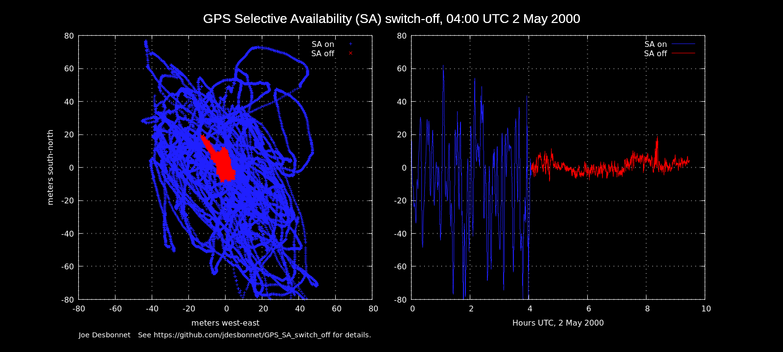
Summary: This article explains how to interface the Texas Instruments TMP006 non-contact IR temperature sensor evaluation module (TMP006EVM) to a Linux computer using the Bus Pirate from Dangerous Prototypes. A small Java program has been written which queries the TMP006 registers using the Bus Pirate, calculates the object temperature and outputs to the screen. Some basic theory of operation is explained and a temperature vs time charts from a cooling mug of coffee and the sky at sunset is presented.
Texas Instruments (TI) recently announced the TMP006, infrared thermopile temperature sensor – ideal for non-contact temperature measurements in the range -40°C to +125°C. The sensor costs just $1.50 in quantity. As with most TI parts, an evaluation kit (TMP006EVM) is available, but at the significantly higher price of $50.

- a TMP006 sensor mounted on a PCB module with a 10 pin header for I2C lines and power
- a SM-USB-DIG: a general purpose USB to I2C/SPI interface which TI use for other evaluation modules also.
The kit also comes with a USB memory stick with the evaluation software, plastic protective case/cover for the SM-USB-DIG and TMP006 module, a USB extension cable, and 30cm ribbon cable suitable for separating the SM-USB-DIG and TMP006 module.
But I use Linux.
My first idea was to write a Linux driver for the SM-USB-DIG. This sub-project has advanced quite a bit, and thanks to a helpful post by a TI employee the protocol has been decoded.... but it isn't returning reliable data just yet.
To expedite matters, I have set the SM-USB-DIG aside for the moment, and turned to the handy Bus Pirate instead.

The TMP006 communicates with the world using I2C/SMBus. Four pins from the TMP006EVM module header (H1) need to be connected:
- H1 Pin 1: I2C SCL connects to the Bus Pirate CLK
- H1 pin 3: I2C SDA connects to the Bus Pirate MOSI
- H1 pin 6: Vcc (3.3V) connects to the Bus Pirate 3.3V
- H1 pin 8: Gnd connects to the Bus Pirate GND.
- Register 0x00: 16 bit signed voltage output from the thermopile (read only)
- Register 0x01: 14 bit die temperature sensor (read only)
- Register 0x02: configuration (read/write)
- Register 0xFE: manufacturer ID (read only, always 0x5449)
- Register 0xFF: device ID (read only, always 0x0060)
The object temperature is a function of the die temperature and the thermopile voltage output. It's not a simple function – some math is involved which is documented in the TMP006 Users Guide, page 10.
To test, connect to the Bus Pirate, enter I2C mode, select 100kHz speed (although slower speeds will be fine too), apply power to the 3.3V line ('W' command) and enter the following command:
[0x80 0xFE [0x81 r r]
All going well the following response should be received:
I2C> [0x80 0xfe [0x81 r r]
I2C START BIT
WRITE: 0x80 ACK
WRITE: 0xFE ACK
I2C START BIT
WRITE: 0x81 ACK
READ: 0x54
READ: ACK 0x49
NACK
I2C STOP BIT
I2C>
This command will read register 0xFE (the manufacturer code) and should return 0x5449.
The normal Bus Pirate interface is written with human interaction through a terminal emulator in mind. Which is great for debugging stuff, but not so handy if a computer program is to be controlling the Bus Pirate. Fortunately, for direct computer control, a binary mode is also available.
I wrote this Java program which uses the Bus Pirate's binary I2C mode to continuously query the TMP006 die temperature and thermopile voltage registers and calculate the temperature of the object in front of the sensor. The RXTX Java IO library is required (available as the librxtx-java package in Ubuntu). [I can re-write this for Python or C. Leave a comment at the end of the post if you're interested in seeing this implemented in another language].
Compiling and running the Java program:
javac TMP006.java
java TMP006 /dev/ttyUSB4 > tmp006.dat
Replace /dev/ttyUSB4 with what ever device the Bus Pirate is connected to. If all goes well you should see the data that looks like this in tmp006.dat (use tail -f tmp006.datto view the log file in real time.
1309198469685 65421 2956 23.09375 24.638878222595167
1309198471555 65422 2956 23.09375 24.66207367078897
1309198473401 65423 2956 23.09375 24.68526379750324
1309198475244 65420 2956 23.09375 24.61567745003481
The columns are:
- Time stamp (milliseconds)
- 16 bit value from register 0x00
- 16 bit value from register 0x01
- Tdie (degrees C)
- Tobj (degrees C)
This gnuplot command will generate a nice chart from the data:
plot 'tmp006.dat' using 1:5 title 'Tobj (C)', \
'tmp006.dat' using 1:4 title 'Tdie (C)'
Theory of operation
Every object emits a characteristic electromagnetic radiation called "black body radiation". The spectrum depends (among other things) on the object's temperature. This is the phenomenon that causes 'red hot' objects to glow a dull red and 'white hot' objects to glow bright yellow/white. Objects at human temperatures also glow, but in the far infrared part of the spectrum which is not visible to the human eye.
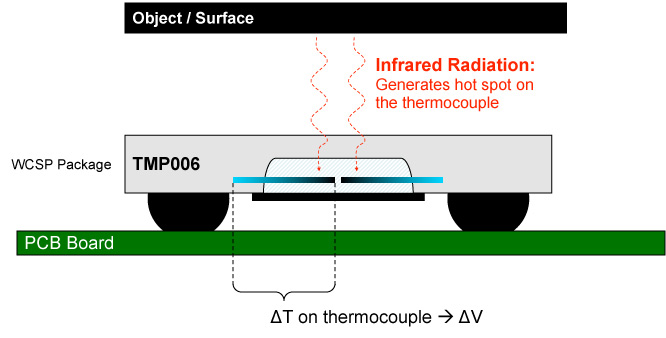
The above chart shows the black body radiation spectrum for melting ice (blue), human skin temperature (red) and a typical mug of coffee (green). The spectrum curves are derived using Plank's Law. Also shown is the TMP006's area of sensitivity (4µm to 8µm [1][2]) and the location of the visible part of the electromagnetic spectrum.
The TMP006 measures the intensity of IR radiation in the 4µm to 8µm region of the spectrum using the Seebeck effect. The measuring circuit built into the the chip/sensor converts the intensity of incident radiation into a voltage which is reported back to the application. Using this voltage, and the temperature of the sensor itself a good estimate of the temperature in front of the sensor can be calculated. The necessary equations are detailed in the TMP006 Users Guide, page 10.
Two things to note. The sensors field of view is a solid angle extending 30 degrees from the normal. Beyond that the sensitivity falls off sharply. Also it is assumed that the emissivity of the target object is reasonably high (> 0.7). Objects such as wood, skin, water and generally anything that's not very white or shiny has a high emissivity and can be measured this way. To get a good reading on shiny metal surfaces that have very low emissivities, it's recommended to cover the area being measured with black tape or paint a patch with black paint.
Some results
This is a chart of the measured temperature of a mug of coffee left cooling. There is approx one temperature sample taken every second. As one would expect, this is a classic Newtons Law of Cooling curve.
This next chart is a temperature vs time chart of the sensor looking up at a cloudless sky (a rare day in the west of Ireland!). I was a little surprised by the results: I expected to see colder temperatures. My other IR thermometers report temperatures well below 0°C when pointing at the sky (away from the sun). Some buildings were in the sensor's field of view which might explain the higher than expected temperatures.

Conclusion
The TMP006 looks like a useful sensor. Looking at TI's promotional material for it, it would seem that they have the mobile devices market in mind. Being able make an instant temperature measurement would certainly be a useful feature for high end smart phones. Also it has a digital interface removing the need for analog signal conditioning and ADC, thus simplifying design and reducing component count.The volume price of just $1.50 seems very reasonable. Unfortunately the tiny 1.6mm square WCSP (Wafer level Chip Scale Package) and the stringent PCB layout guidelines [3] make this device difficult to use unless you have access to a advanced surface mount soldering workshop. Hopefully this sensor will be available on a breakout board in the near future.
Footnotes and references
[1] TMP006 Users Guide (SBOU107), page 2.[2] Discussion on TMP006 at TI forums
http://e2e.ti.com/support/other_analog/temperature_sensors/f/243/t/117229.aspx
[3] TMP006 Users Guide (SBOU107), Layout Guidelines, page 6.
Diagram on principles of operation taken from TI promotional material.